Rows and columns and histograms
Warning: post below is more technical than usual. I finally figured out something which had been confusing me for a long time, although I’m sure it’s obvious to others. My explanation below is partly to solidify my own understanding and partly in case I’m not the only person confused about this.
I have been working with astronomical images for just about half my life now. Usually these come in FITS format, with the conventions that the pixels are identified in a Cartesian way: x increases to the right along the horizontal axis, and y increases to the top along the vertical axis, with pixel (1,1) in the lower left of the image. Pixel centers are integer coordinates. My understanding is that neither of these conventions is universal.
Recently I was trying to plot a 2-D histogram using the histogram2d function in numpy. The idea of a
2-D histogram is that you have a set of points in the xy plane, you divide that plane
into bins (which you can also think of as pixels), and count how many points are in
each bin (this number would be the pixels’ value). The documentation explains how to
use the function and gives the helpful information that
the histogram does not follow the Cartesian convention where x values are on the abscissa and y values on the ordinate
axis. Rather, x is histogrammed along the first dimension of the array (vertical), and y along the second dimension of the array
(horizontal).
What does this helpful information mean? It’s a reminder that arrays in Python do not follow
the image conventions that I described above. In Python, array indices are written in
this order: [row,column] and when printed, position [0,0] is in the upper left.
The array axes are defined such that axis 0 is rows and axis 1 is columns, meaning that if data
is an array and you do something like data.mean(axis=0), you are averaging each column over all
rows, in other words along the vertical direction. If you do data.mean(axis=1), you are averaging
each row over all columns, in other words along the horizontal direction.
This lovely figure from the Software Carpentry Python lesson helps explain:

histogram2d constructs an array by the procedure described above.
But the helpful information tells you that you can’t just plot the resulting array as an image over the (x,y) data points,
because the array has the axes interchanged, and it starts at the upper left rather than lower.
To plot the output of histogram2d with the data points, you have to either:
- plot it as an image but accept that you get your
yvalues on the horizontal axis - transpose it using
T(see Dave’s Matplotlib Basic Examples) - or rotate it and flip it along one axis (same as transposing; see 2-D Histogram)
Regardless of which of these methods are used, you also need to use origin=lower in matplotlib.imshow to get
(0,0) in the lower left.
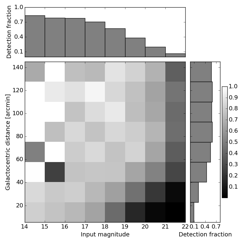
I figured this out because I was trying to make a fancy plot with the 2-D histogram in the middle
and the associated 1-D histograms along its sides, a bit like
this,
which is based on this matplotlib example
The way to make the 1-D histograms is by summing
the 2-D histogram along one of the axes. Summing on axis=0 involves summing each column along rows,
so that should give you the number of objects as a function of your y variable, and summing on
axis=1 should give you the number as a function of x.
Here is a figure which uses this approach, and the code that produced it (this code actually required two 2-D histograms because of what I’m computing here; here is a somewhat simpler version).
I hope you find this useful; comments and/or corrections are welcome, either below or via pull request here.